Binning demonstration on locally generated fake data
In this example, we generate a table with random data simulating a single event dataset. We showcase the binning method, first on a simple single table using the bin_partition method and then in the distributed method bin_dataframe, using daks dataframes. The first method is never really called directly, as it is simply the function called by the bin_dataframe on each partition of the dask dataframe.
[1]:
import sys

import dask
import numpy as np
import pandas as pd
import dask.dataframe

import matplotlib.pyplot as plt

sys.path.append("../")
from sed.binning import bin_partition, bin_dataframe
Generate Fake Data
[2]:
n_pts = 100000
cols = ["posx", "posy", "energy"]
df = pd.DataFrame(np.random.randn(n_pts, len(cols)), columns=cols)
df
[2]:
| posx | posy | energy | |
|---|---|---|---|
| 0 | -1.597617 | -0.543767 | 0.729540 |
| 1 | -1.765663 | -1.610388 | -1.131555 |
| 2 | 2.330603 | 2.251475 | -1.256111 |
| 3 | -0.729069 | -0.330417 | 1.571411 |
| 4 | 1.003576 | 1.423138 | 0.859336 |
| ... | ... | ... | ... |
| 99995 | -0.063640 | 0.004117 | -0.801435 |
| 99996 | -1.198671 | -0.618133 | 1.084128 |
| 99997 | -0.085724 | 2.608801 | 0.226714 |
| 99998 | 0.237666 | 1.075434 | -0.435475 |
| 99999 | -0.633201 | 0.019438 | -0.329833 |
100000 rows × 3 columns
Define the binning range
[3]:
binAxes = ["posx", "posy", "energy"]
nBins = [120, 120, 120]
binRanges = [(-2, 2), (-2, 2), (-2, 2)]
coords = {ax: np.linspace(r[0], r[1], n) for ax, r, n in zip(binAxes, binRanges, nBins)}
Compute the binning along the pandas dataframe
[4]:
%%time
res = bin_partition(
    part=df,
    bins=nBins,
    axes=binAxes,
    ranges=binRanges,
    hist_mode="numba",
)
CPU times: user 1.24 s, sys: 39.5 ms, total: 1.28 s
Wall time: 1.43 s
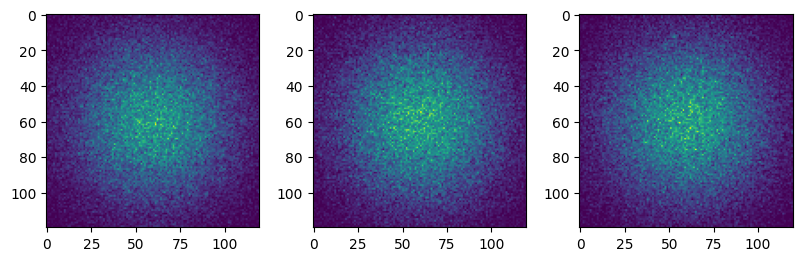
[5]:
fig, axs = plt.subplots(1, 3, figsize=(8, 2.5), constrained_layout=True)
for i in range(3):
    axs[i].imshow(res.sum(i))
Transform to dask dataframe
[6]:
ddf = dask.dataframe.from_pandas(df, npartitions=50)
ddf
[6]:
Dask DataFrame Structure:
| posx | posy | energy | |
|---|---|---|---|
| npartitions=50 | |||
| 0 | float64 | float64 | float64 |
| 2000 | ... | ... | ... |
| ... | ... | ... | ... |
| 98000 | ... | ... | ... |
| 99999 | ... | ... | ... |
Dask Name: from_pandas, 1 graph layer
Compute distributed binning on the partitioned dask dataframe
In this example, the small dataset does not give significant improvement over the pandas implementation, at least using this number of partitions. A single partition would be faster (you can try…) but we use multiple for demonstration purposes.
[7]:
%%time
res = bin_dataframe(
    df=ddf,
    bins=nBins,
    axes=binAxes,
    ranges=binRanges,
    hist_mode="numba",
)
CPU times: user 401 ms, sys: 521 ms, total: 922 ms
Wall time: 509 ms
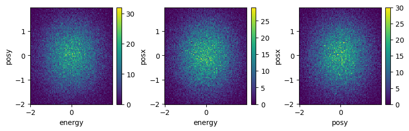
[8]:
fig, axs = plt.subplots(1, 3, figsize=(8, 2.5), constrained_layout=True)
for dim, ax in zip(binAxes, axs):
    res.sum(dim).plot(ax=ax)
[ ]: